ShowMe - Atwood's Pulley (massless pulley)

1. The applet does not give accelerations directly, but it does provide sufficient information for you to calculate the acceleration of the masses. The information needed to do this is the time (t) and the distance traveled by mass 1. This data is given in the upper left-hand corner of the applet display panel. As an example, adjust the size of the masses to be 300 g and 700 g respectively. Next, click "Play" and wait. The masses will begin to move. Wait until the animation stops. The displacement of mass 1 and the time taken for this displaement to occur appear in the upper left corner of the panel.
2. In this case, the duration of movement was 0.760 s and the distance that mass 1 traveled was 1.133 m.
3. If we recall that the distance-time relationship for an object accelerating from rest is , and that we can rearrange this equation to give us , then it is a straight-forward calculation to show that acceleration a = 3.92 m/s².

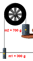
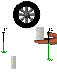
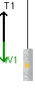
1. A Free Body Diagram (FBD) for each mass can be produced by pressing the Free Body Diagram control button. When you do this, the images of the masses will fade slightly and force vectors representing the weight and tension will appear (see the figure below). The hand indicates that mass 2 is held before release. In this case, the tension in the strings is entirely due to the weight of mass 1.

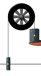
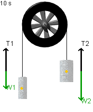
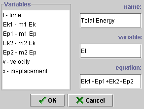
2. Note that when you click "Play", the supporting hand disappears and the masses move. The tensions shown in the strings will change.

3. The tensions in the supporting strings are not shown. They can be easily calculated, however, by first finding the acceleration for each mass and then applying Newton's second law . For example, in the previous discussion of acceleration, we determined that mass 1 was accelerating upward at 3.92 m/s². If we use the FBD for mass 1 (shown on the left) and if we assign up as the positive direction, the following force-equation is implied:
   

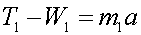
   Since ,we find that

   
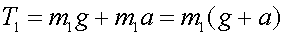
   Since mass 1 = 0.300 kg and a = 3.92 m/s², we find that both T₁ and T₂ are equal to 4.12 N .

1. When you run the Atwood applet, you will see a horizontal line labeled "Ep Reference". This line is used to define a position at which the two masses have zero potential energy. You can capture this line by positioning the mouse over it and then, holding down the left-mouse button, drag up or down. When you "capture" the line, it will fade slightly as shown below.
   To illustrate this, adjust the masses so that mass 1 = 300 g and mass 2 = 700 g.

EP Reference not yet "captured" by the mouse

EP Reference has been"captured" by the mouse

2. Each mass has a yellow dot that indicates its centre of mass. To see how to use the EP Reference line effectively, position the EP Reference line so that it passes through the yellow dot (center of mass) for mass 1.

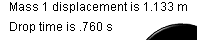
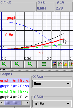
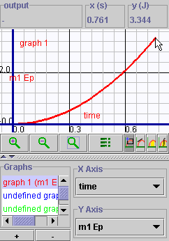
3. Click "Play", wait until the motion stops, and then click "View Graph". Produce a graph with time on the x-axis and the potential energy of mass 1 (m1 EP) on the y-axis. You should see a graph very similar to the one below. Note that the potential energy for mass 1 starts at zero - just as we would expect, since we put the EP Reference line at this point. Also note that when the motion stopped, mass 1 had ascended to a point 1.133 m above the reference line. Since 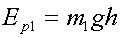(where E_p1 is the potential energy of mass 1 and h is the height through which it moved), we can insert the numbers to find that:

E_p1 = (0.300 kg)(9.81 m/s²)(1.133  m) = 3.33 J .

You can verify this calculation by inspecting the graph below.

1. Set up the Atwood pulley so that mass 1 = 250 g and mass 2 = 750  g. Position the EP Reference line at the centre of mass for the 250  g mass. You should have a setup similar to the one shown below.
2. Press "Play" and note the distance through which each mass has moved when the motion stops. You should see that mass 1 rose 1.134 m while mass 2 dropped 1.134 m.

3. Next, click "View Graph" and prepare the following 4 graphs:
   • time - mass1 E_p
   • time - mass 2 E_p
   • time - mass1 E_k
   • time - mass 2 E_k

   You should see something similar to what appears below.

4. You may need to resize the graph to inspect the graph and verify that the values appearing are correct. For example, since mass 1 is 0.250 kg and rose through 1.134 m, it is easy to see that:

= (0.250 kg)(9.81 m/s²)(1.134 m)

= 2.78 J

By clicking on graph 1 and positioning the mouse overtop of this graph, it is easy to see that after 0.684 s, the potential energy of mass 1 is 2.78 J. You can find the other energies by repeating this process for the appropriate graph.

1. A powerful feature of the grapher is the ability to create new variables that are not listed in the original drop-down menu of variables to plot. Since we plotted the potential and kinetic energy terms for the two masses in the previous example, it is instructive to ask "What would the sum of all of these terms look like?". To do this, close the graph and click the data collection button (). A drop-down menu appears (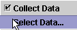) - choose "Select Data". A dialogue box like the one shown below will appear. Since you want to create an expression that does not appear in those listed, click "Add".

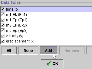2. After clicking "OK" (), a new dialogue box opens. Fill in the blank spaces exactly as shown below. Be very careful to type the variables exactly as they appear in the list of available variables. You only can build equations out of the pre-existing set of variables. When you are finished, click "OK". You now have created a variable called "Total Energy" and it is available for plotting on the graph.

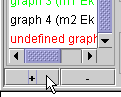
3. To plot "Total Energy", you will need to add one more equation to the graph. Press the small "+" button at the bottom of the graph panel (as shown below). A new graph, labeled "undefined graph" appears at the bottom of the previous list of 4 graphs.

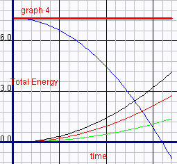
4. Proceed as you would with any other graph. Note that this time when you click the "X axis" or "Y axis" buttons, a new variable appears in the list - "Total Energy". Select time for the x-axis and Total Energy for the y-axis.
5. Next, click "Reset" and then click "Play". This will update the graph, and also use the newly defined variable Total Energy. When finished, you should see a graph very similar to the one below.