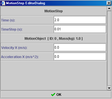
- A motion script is a set of instructions that you enter in the 1D
Non-Uniform Motion Builder Graphing (pos, vel, acc) applet by clicking
"Add" (
 )
and then filling out the information required in an information window
that opens. A sample window is shown here. There are four pieces of
information that you can alter:
)
and then filling out the information required in an information window
that opens. A sample window is shown here. There are four pieces of
information that you can alter:
- Time (s): this is the amount of time for the motion in this script
- TimeStep (s): Time step is the interval of time between successive
calculations of the motion. If you are unsure about this then it
is best to leave it at the default value of 0.01 s. Normally
the time step should be about 1 percent of the entire time for the
motion. For example, if you wanted the motion to occur over a span
of 100 s, then the time step should be increased to be about
0.10 s. Too big a time step will result in a drop of precision
in the simulation of the motion. Too small a time step will result
in the generation of too much "data" when the applet does
its calculations.
- Velocity X (m/s): set this for whatever value is needed.
(NOTE: do not put units with your values - they are already included as shown. )
- Acceleration X (m/s^2): set the acceleration here.
- Time (s): this is the amount of time for the motion in this script
- Click "OK" (
 )
to close the menu and save the motion script.
)
to close the menu and save the motion script.
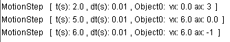
- You can make as many scripts as you wish by simply clicking the "add script" button and supplying the required information. The figure shown on the right shows three scripts. The information for each script is shown. The total time required for the entire motion will just be the sum of the times for each script. In this example the total time will be 2.0 s + 3.0 s + 2.0 s = 7.0 s.
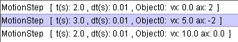
- As an example, create a motion that has the following three
parts, each described by a script:
- A ball accelerates from rest at 3 m/s2 for 2 s.
- It coasts at a constant speed of 6 m/s for 5 seconds.
- The ball begins to decelerate at -1 m/s2 for 6 s.
Enter this information into MotionBuilder. When finished, your motion scripts should appear in the Motion Script Display Window and look like the following
 )
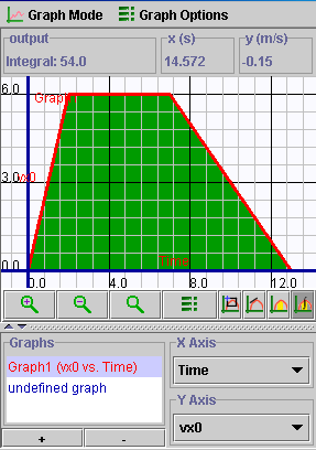
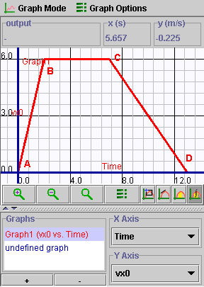
and position the mouse at t = 0 s. Hold down the left mouse button
and drag across the graph to t = 13 s. As you do this, the area
between the time axis and the graph is painted green and the output
panel now reads Integral and gives a running value for the area that
you are creating. If you paint all the way to t = 13 s you will
see that the size of the green area is equal to 54.0 m. Note: the
grapher will not supply units for this - you must recognize that the
area must have units of (m/s) X (s) = m and put these in yourself!
So the distance traveled in this motion is 54.0 m.
)
and position the mouse at t = 0 s. Hold down the left mouse button
and drag across the graph to t = 13 s. As you do this, the area
between the time axis and the graph is painted green and the output
panel now reads Integral and gives a running value for the area that
you are creating. If you paint all the way to t = 13 s you will
see that the size of the green area is equal to 54.0 m. Note: the
grapher will not supply units for this - you must recognize that the
area must have units of (m/s) X (s) = m and put these in yourself!
So the distance traveled in this motion is 54.0 m.